Why Your DB Chatbot Needs a Knowledge Graph, Not Just a Schema

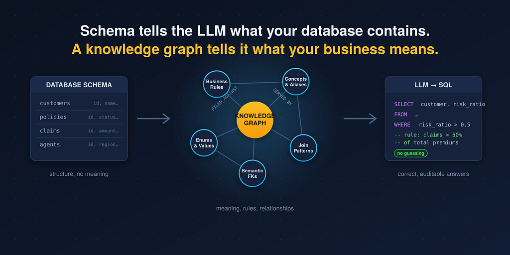
Large language models have made natural-language-to-SQL feel almost solved. Wire up an LLM, hand it your database schema, and business users can ask questions in plain English. Except it isn’t solved — because the moment a user asks a question that depends on business meaning rather than table structure, the schema-only approach falls apart.

This post walks through an architecture for a Text2SQL chatbot that grounds the LLM in a knowledge graph built from the database schema and enriched with business semantics. The result is a system that doesn’t guess what “high-risk customers” means — it knows, because the definition lives in the graph.

The Anatomy of a Text2SQL Chatbot

Before getting to the knowledge graph, it helps to see the full design flow of an LLM-enabled Text2SQL chatbot. The pipeline has six stages:

1. User Query Capture. The raw question comes in and passes through input sanitation, query length validation, and guardrails before anything else happens.

2. Context Assembly. This is the heart of the system — and the stage this whole post is about. Here the system gathers everything the LLM needs to answer well: the query intent, the database schema context, conversation history, few-shot samples, and the expected response format.

3. LLM Request Payload. The assembled context becomes a structured request: a system message carrying the domain context, the user message, and model parameters.

4. LLM Response Processing. The model’s output is parsed and validated, the generated SQL is extracted and cleaned, and the system performs a confidence assessment and extracts the model’s reasoning.

5. Security and Execution. Before anything touches the database, the generated SQL goes through query validation, forbidden-operation blocking (no DROP, no DELETE), access validation, and resource usage limits. Only then is the query executed.

6. Response Formatting. Results come back as data visualizations, a natural-language summary, and any additional context the user needs.

Most teams get stages 1, 3, 4, 5, and 6 right. Stage 2 — context assembly — is where quality is won or lost.

The Problem: Schema Alone Doesn’t Carry Meaning

Consider a working example from an insurance analytics domain, with a familiar relational model: customers, policies, claims, and agents, connected by foreign keys.

A user asks: “Show me our high-risk customers.”

What the LLM receives with basic (conventional) context

1. 1.Tables: customers, policies, claims
2. 2.Foreign keys: policies.customer_id → customers.customer_id, policies.agent_id → agents.agent_id, claims.policy_id → policies.policy_id

And here is the LLM’s actual reasoning under that context:

The user is asking for ‘high-risk customers’ but I don’t see any ‘risk’ column in the customers table. Let me look at the schema again… Maybe ‘high-risk’ means customers with many claims? Customers with high claim amounts? Some risk score column that might exist? I’ll guess that high-risk means customers with claims, but I’m not sure about the specific criteria.

The model is guessing. It might invent WHERE risk > 0 against a column that doesn't exist, or hallucinate WHERE customer_type = 'high-risk'. The schema is structurally complete and semantically empty.

What the LLM receives with knowledge-graph-enhanced context

Instead of a bare schema, the LLM receives a complete domain knowledge graph: entities, business relationships, business rules, and business context. Its reasoning transforms:

This is asking for customers who meet the business definition of ‘high-risk’ based on the risk assessment rules provided. According to the domain knowledge: high-risk = customers with total claims > 50% of total premiums. Need to calculate risk ratio: Total Paid Claims ÷ Total Premiums. Only include active policies. Only count approved/paid claims (not pending or denied). Filter for risk ratio > 0.5. Return customer identification, metrics, and risk ratio, ordered by highest risk first to prioritize attention.

Same model. Same question. The difference is entirely in the context.

Three more examples of the same failure mode

“Find expired policies that need renewal.” Basic context sees end_date and status columns and generates WHERE end_date < TODAY() — ignoring status logic and missing the grace-period rule entirely. The knowledge graph understands the policy lifecycle (Active → Expired → Renewable vs. Cancelled) and knows the rule "expired policies are renewable within 30 days," producing WHERE status = 'Expired' AND end_date BETWEEN (TODAY() - 30) AND TODAY().

“Show customers eligible for multi-policy discounts.” Basic context has no concept of a multi-policy discount and falls back to counting policies (HAVING COUNT(*) > 1). The knowledge graph carries the actual eligibility rule — the discount requires an Auto + Home or Auto + Life combination — and generates logic that checks specific policy-type combinations.

“Find our most profitable customer segments.” There is no profitability column, so the basic approach might sort by premium_amount DESC — which is simply wrong. The knowledge graph knows profitability = total premiums − total claims paid, joins policies and claims for the calculation, and segments by policy types and customer characteristics.

The pattern across all four: business vocabulary rarely maps one-to-one to columns. “High-risk,” “needs renewal,” “eligible for discount,” “profitable” — these are derived concepts defined by rules, and those rules have to live somewhere the LLM can see them.

The Knowledge Graph Ontology: Two Layers

The knowledge graph is organized as an ontology with two layers.

The SQL structure layer captures the physical database as-is: datasets, schemas, tables, and columns. This is what conventional Text2SQL already provides.

The business semantics layer sits on top and integrates everything the schema can’t express:

1. 1.Concepts — what business terms like “policy type” or “risk ratio” actually mean
2. 2.Rules — computable business logic (thresholds, tiers, eligibility criteria)
3. 3.Enumerations — allowed values and what each one means
4. 4.Column and table synonyms / aliases — the vocabulary business users actually use
5. 5.FK relations with semantics — not just that keys join, but why
6. 6.Join patterns — pre-validated multi-table paths for common analytical questions
7. 7.Query patterns — reusable shapes for recurring question types

The structural layer answers “what exists?” The semantic layer answers “what does it mean, and how do we use it?”

The Construction Pipeline

Building the graph is a repeatable pipeline, not a one-off modeling exercise:

Step 1 — Semantic modelling. Start from the SQL database (PostgreSQL or BigQuery): tables, columns, keys, indexes. Model the domain as an OWL ontology (classes, properties, relationships) and define R2RML mapping rules that translate relational structures into graph form. This is implemented in Python with RDFLib.

Step 2 — Knowledge graph materialization. The mappings produce an RDF knowledge graph that is fully SPARQL-queryable. It can be hosted in a triple store such as Jena Fuseki, or represented in Neo4j, with artifacts persisted in cloud storage.

Step 3 — Semantic enrichment. This is where the business layer gets attached: aliases, enumerations, value ontologies, business rules, join snippets, and guardrails. Critically, this includes user-enhanced content — domain experts contribute definitions the schema could never carry. Again Python with RDFLib and SPARQL.

Step 4 — Text2SQL at runtime. When a question arrives, context generation runs SPARQL queries against the graph to pull exactly the relevant slice of domain knowledge into the LLM system prompt. The call to the LLM is system prompt + user query; the model generates SQL, which is validated and executed. The chatbot front end is built with Streamlit and Google ADK.

The key architectural insight: the knowledge graph is queryable context, not a static document. SPARQL lets the system assemble a focused, per-question context rather than stuffing the entire domain model into every prompt.

The Building Blocks, Concretely

Abstractions are easy to nod along to; the deck grounds each enrichment type in real JSON from the insurance domain. Here’s what each one looks like and why it matters.

1. Business Concepts

A concept ties a business term to its physical column and its meaning:

{ "business_concept": { "name": "policy_type", "related_terms": ["coverage_classification", "product_category"], "column": { "table": "insurance_policies", "name": "policy_type", "type": "STRING", "required": true, "distinct_values": 5 }, "aliases": ["coverage_type", "insurance_type", "product_type", "coverage"], "sensitivity": "low" }}Policy type categorizes policies by coverage classification and product type. The concept records the technical facts (required STRING field, 5 distinct values across 102 policies, never null) alongside the business usage: portfolio management, risk segmentation, regulatory filing, and product popularity analysis. And it lists the natural-language terms users actually say — “coverage type,” “insurance type,” “product type,” or just “coverage” — so any of them resolves to the right column.

2. Business Rules

Rules make derived concepts computable. Premium segmentation, for example:

{ "premium_segmentation_rules": { "category": "premium_segmentation", "applies_to": "insurance_policies", "tiers": [ { "rule_id": "rule_18", "tier": "Budget", "logic": "premium <= 2000", "range": "≤ $2,000" }, { "rule_id": "rule_19", "tier": "Standard", "logic": "premium BETWEEN 2000 AND 5000", "range": "$2,000 - $5,000" }, { "rule_id": "rule_20", "tier": "Premium", "logic": "premium > 5000", "range": "> $5,000" } ] }}When someone asks about “budget-tier policies,” the LLM doesn’t need to invent a threshold — the rule carries the exact SQL logic. These rules serve pricing strategy, marketing campaigns, and portfolio analysis, and the same mechanism encodes the “high-risk” definition from earlier.

3. Aliases

Business users don’t know table names. The insurance_customers table carries 12 aliases spanning three registers:

1. 1.Insurance-specific: policyholders, policy_holders, insured, insureds
2. 2.Business relationship: clients, customers, customer_base
3. 3.General: individuals, people, members, subscribers, account_holders

Whether a user says “show me our policyholders” or “list all members,” the query resolves to the same table. Nobody has to learn the physical schema to ask a question.

4. Enumerations

Enumerations declare a column’s allowed values and what each means. insurance_claims.claim_status accepts exactly five values:

1. 1.Approved — claim approved for payment
2. 2.Under_Review — under investigation or review
3. 3.Pending — awaiting additional information
4. 4.Denied — rejected
5. 5.Settled — paid and closed

This matters enormously for correctness. Remember the high-risk rule: only approved/paid claims count. Without the enumeration, an LLM would happily sum pending and denied claims into a risk ratio and produce a confidently wrong answer.

5. Foreign Keys with Semantics

A conventional schema says insurance_claims.policy_id → insurance_policies.policy_id. The knowledge graph says more:

{ "type": "ForeignKey", "from_column": "insurance_claims.policy_id", "to_column": "insurance_policies.policy_id", "relationship_type": "FILED_AGAINST", "cardinality": "MANY_TO_ONE", "meaning": "Each claim is filed against one policy", "join_hint": "Essential join for claims analysis"}The relationship type FILED_AGAINST teaches the LLM that claims are legally and contractually tied to policies — not just technically linked. This prevents a whole class of hallucinations where the model tries to join claims directly to customers or agents. It learns that policies are the required intermediary: for “customer claim history” or “loss ratio” questions, the path is customers → policies → claims, with policy context (type, premium, coverage) included because claims data alone isn’t sufficient for meaningful analysis.

6. Join Patterns

For common multi-hop questions, the graph ships pre-validated join paths:

{ "type": "JoinPattern", "label": "Customer→Agent", "description": "Customer to agent join via policy relationship", "join_pattern": "insurance_customers c JOIN insurance_policies p ON c.customer_id = p.customer_id JOIN insurance_agents a ON p.agent_id = a.agent_id", "usage": "Use for queries involving customer-agent relationships", "purpose": "Links customers to their servicing agents through policies", "join_type": "INNER", "directionality": "many-to-many", "example_query": "Show which agent serves each customer"}The purpose statement — “links customers to their servicing agents through policies” — encodes a business fact: agents serve customers by selling them policies, so the relationship is mediated, and a customer can have multiple agents if they bought different policies from different ones. When a user asks “which agent handles this customer?” the LLM doesn’t have to derive the three-table path; it applies a known-good pattern. This is critical for agent performance analysis, customer service routing, and commission calculations.

Why This Architecture Works

Stepping back, the design succeeds for a few reinforcing reasons:

It moves ambiguity resolution out of the model and into the data. Rather than hoping the LLM guesses your business definitions correctly, the definitions are explicit, versioned artifacts in the graph. Guessing becomes lookup.

It’s queryable, so context stays focused. Because the graph is RDF and SPARQL-queryable, context generation retrieves only what’s relevant to the question at hand — not the entire domain model — keeping prompts sharp and token budgets sane.

It uses standards. OWL for the ontology, R2RML for relational-to-graph mapping, RDF/SPARQL for storage and retrieval. The stack (RDFLib, Jena Fuseki or Neo4j, Streamlit + Google ADK, PostgreSQL/BigQuery) is composed of proven, interoperable components rather than a bespoke format.

It has a place for human knowledge. The semantic enrichment step explicitly incorporates user-enhanced content. Domain experts — the people who know that a multi-policy discount requires Auto + Home — have a structured channel to encode that knowledge once, and every subsequent query benefits.

It keeps the safety rails. The knowledge graph improves generation quality; the surrounding pipeline still enforces SQL validation, forbidden-operation blocking, access control, and resource limits before execution. Better context and defense-in-depth are complementary, not alternatives.

The Takeaway

Text2SQL accuracy is not primarily a model problem — it’s a context problem. A schema tells the LLM what your database contains; a knowledge graph tells it what your business means. The gap between those two is exactly the gap between “I’ll guess that high-risk means customers with claims” and a correct, auditable risk-ratio calculation with the right status filters and the right joins.

If your Text2SQL chatbot is hallucinating columns, misjoining tables, or inventing definitions for business terms, the fix isn’t a bigger model. It’s a knowledge graph: model the schema as an ontology, enrich it with concepts, rules, aliases, enumerations, semantic relationships, and join patterns, and let SPARQL assemble precise context per question. The LLM stops guessing — and starts reasoning with your business’s actual knowledge.